The last month or so I have been burning the candle at both ends, investigating dataset properties and their relationship with how statistical models operate. It’s been rather fascinating to be able to adjust aspects of a dataset and see how it impacts different modeling frameworks (both Bayesian and Frequentist). It’s also led me to some pretty important findings related to the ways in which these frameworks can obscure or inflate statistical results.

What is data topology?

To give a bit of background, “topology” refers to the shape of something, i.e. its dimensions and its surface. A key observation is that modeling frameworks make assumptions about the data they are dealing with, specifically in terms of geometry. If you consider that a data point is essentially an observation or measurement, this allows it to be quantified or given a numeric value. There are various ways of turning a data point or observation into a number, and depending on how this is done, you develop a set of matrices or numeric vectors that relate your single data point to other data points in the problem space.

Topology is the shape of how that data is represented numerically, or how it is connected to the other data in the dataset, which then affects the kinds of relationships you can observe and estimate. There is an emerging field of mathematics known as Topological Data Analysis, applied in various fields to identify important features of a dataset. As an example of one possible shape of data, here is a side-by-side comparison of two different datasets, one from biology and one from linguistics. These are phylogenies - measurements of relatedness between languages, expressed as “trees”.

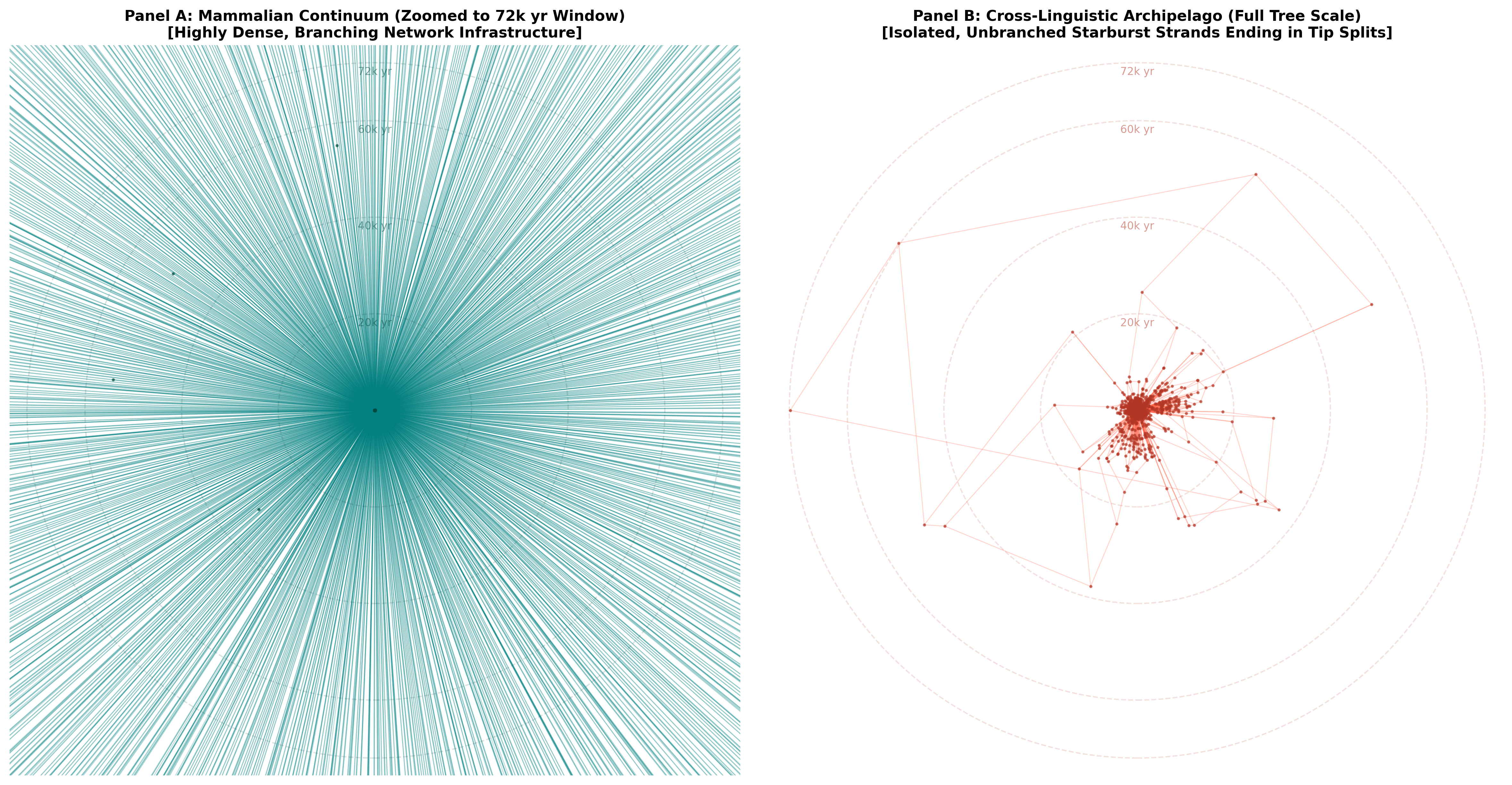
In this image the biological tree is actually just part of the existing “mammals” tree for vertebrates. This vertebrate phylogeny (green) contains roughly 2k data points/nodes, which is about the same number as found in the linguistic dataset that is visualized next to it (in red). I’ve also set the time depth at 75k years to match the depth of the linguistic tree. From this comparison we can clearly see that a biological phylogeny is incredibly dense. It also has an extreme time depth, with a proposed evolutionary history of hundreds of millions of years. Language, on the other hand, has many fewer observations and it is extremely difficult to reconstruct any family tree beyond 2,000 years ago or so, meaning that this graphic represents the absolute limits of our hypotheses regarding language relatedness.

Problems with sparse datasets

Differences between biological and linguistic or cultural datasets are often framed in terms of “sparsity”, which generally refers to a lack of observations - either low numbers/counts or missing data points. The lack of data can lead to classic problems with generalization and/or erroneous conclusions (false positives). Since much social/behavioral data is based on qualitative observation, this has long been a critique of the field: how do you apply statistical methods to these kinds of limited observations?

The data sparsity problem is parallel to another kind of sparsity, which is network connection. The interconnectedness of datapoints in a dataset (density) may be low or high, which is directly related to how well a statistical model can render judgements about the data itself. When density is low, this is akin to a sparsity problem, and statistical frameworks often struggle to accurately assess the data. In another post, I’ll highlight some of these estimation problems, which apply (in different ways) to both Frequentist (maximum likelihood, fixed parameters) and Bayesian (probability distributions, random parameters) models. Crucially, topological density (network connectedness) can operate at multiple levels, and is a separate concern from traditional sparsity.

The Topological Stability Index and pyTstability

In my investigations over the past month, I realized that I needed a way to quantify these topological properties. There isn’t an existing framework that does this, so I developed a tool. The pytstability package provides a means of assessing how well-connected a dataset is, i.e. the internal Topological Stability of the data. This is a mathematically derived metric based on the properties of a given dataset, assessing both spatial and structural connectivity using coordinate matrices and categorical codes. The Topological Stability Index (TSI) provides researchers with a way of quantifying their dataset’s properties before modeling, highlighting potential estimation issues before they arise and helping to assist with statistical model selection.

Using the package is relatively straightforward, and I provide some examples in the repo that cover biology, culture, and linguistics. Here, I’ll walk you through how you could use it with a linguistic dataset, to illustrate both the spatial and structural components. You can download the relevant files at the repository linked above - as with other tutorials, I assume you have a Python 3.10 environment and some familiarity with writing and running Python scripts (i.e. via a terminal). For a basic setup tutorial, you can follow these instructions.

Installing the package

Installing the package can be done using pip and git from a standard command line interface:

pip install git+https://github.com/lingdoc/pytstability

We then make sure that we have the dataset we want to assess. This can be any kind of spreadsheet file, but you’ll need to convert it into a dataframe, which is most easily done using pandas. In my case, I’ve downloaded the relevant 0573KA feature files and the Glottolog csv file (from the example data/tlu/ directory of the pytstability repo) and placed them into a subdirectory where I’m running my python script.

# import libraries for dealing with files
import os
import pandas as pd

# read in the Glottolog data with spatial coordinates
glottolog_data = "tlu/Glottolog_Languages.csv"
gldf = pd.read_csv(glottolog_data)
# remove languages that don't have spatial coordinates
gldf = gldf.dropna(subset=['latitude', 'longitude'])
# reduce to the following columns
keepcols = ['glottocode', 'macroarea', 'Family_ID', 'longitude', 'latitude']
gldf = gldf[keepcols].copy()

# get the binary-coded feature file
feat_path = "tlu/0573KA/BT_data.txt"
# get the base directory info
feat_id = str(os.path.basename(os.path.dirname(feat_path)))
print(f"\n -> Assessing language feature: {feat_id}")
fdf = pd.read_csv(feat_path, delimiter="\t", header=None, names=["glottocode", "DV", "IV"])

# combine the two dataframes on 'glottocode' so we have it all in one sheet
ling_df = pd.merge(gldf, fdf, on='glottocode', how='inner')
print(f"    Matched {len(ling_df)} languages on the map.")

# get the phylogeny file for this feature (it is a zipped Newick file)
tree_path = "tlu/0573KA/pruned_tree.trees.gz"

# -> Assessing language feature: 0573KA
#    Matched 1744 languages on the map.
#

Assessing topological stability

Now that we have all the data in a single sheet, we can work on estimating the connectivity of the dataset. To do this we import the pytstability package and set it up with some arguments, storing the results in a variable. The only required arguments are the data (assumes a pandas dataframe) and id_col (the individual observations/nodes), so let’s see what happens when we only declare those arguments. When you run the following code it prints out some information in the terminal (default verbose=True).

# import the core calculator function from the package
from pytstability import calculate_densities

# get the metrics
t_metrics = calculate_densities(
    data=ling_df, # the dataframe
    id_col='glottocode' # the id column
)

# -- Data Topology Metrics --
# Spatial Mode       : none (Components: 1)
# Structural Mode    : none (Components: 1 | Optimized Depth: auto)
# Spatial Topology   : κ = nan | P_isolated = nan | S_giant = nan
# Structural Topology: κ = nan | P_isolated = nan | S_giant = nan
# Unified Diagnostic : Topology Stability Index (TSI) = 0.000000
# Critical Ceiling   : Dynamic Danger Horizon (Gamma)   = 0.003466

As you can see, it doesn’t give us much information without data columns defined. We really need to pass it some other arguments regarding the spatial or structural relations in our dataset. In terms of spatial relations, we can give the function either coordinates (latitude, longitude) or categorical groupings (land areas) or both. In the case of structural relations, we can include the path of a tree/phylogeny, or categorical groupings (i.e. families) or both. The tool will try to automatically calculate the most robust relational structure, but you can also configure it manually (see options/examples at the linked repository). Let’s just pass in a mix of features and see what the result is.

# get the metrics
t_metrics = calculate_densities(
    data=ling_df, # the dataframe
    id_col='glottocode', # the id column
    # add spatial coordinate columns
    coord_cols=['latitude', 'longitude'],
    # add spatial category columns (string or list of strings)
    spatial_cats='macroarea',
    # add path to a phylogenetic tree
    tree=tree_path,
    # add structural category column(s)
    struct_cats='Family_ID'
)

# Enforcing Relative Ratio Threshold Optimization (Linguistics Paradigm)...
# Building Matrix (adaptive mode | Ratio 0.50): 100%|████| 1744/1744 [00:01<00:00, 904.59it/s]
# Building Matrix (adaptive mode | Ratio 0.70): 100%|████| 1744/1744 [00:01<00:00, 935.17it/s]
# Building Matrix (adaptive mode | Ratio 0.80): 100%|████| 1744/1744 [00:01<00:00, 937.07it/s]
# Building Matrix (adaptive mode | Ratio 0.85): 100%|████| 1744/1744 [00:02<00:00, 853.07it/s]
# Building Matrix (adaptive mode | Ratio 0.90): 100%|████| 1744/1744 [00:02<00:00, 871.01it/s]
# Building Matrix (adaptive mode | Ratio 0.93): 100%|████| 1744/1744 [00:01<00:00, 903.48it/s]
# Building Matrix (adaptive mode | Ratio 0.95): 100%|████| 1744/1744 [00:01<00:00, 913.98it/s]
# Building Matrix (adaptive mode | Ratio 0.96): 100%|████| 1744/1744 [00:01<00:00, 939.03it/s]
# Building Matrix (adaptive mode | Ratio 0.97): 100%|████| 1744/1744 [00:01<00:00, 938.12it/s]
# Building Matrix (adaptive mode | Ratio 0.98): 100%|████| 1744/1744 [00:01<00:00, 938.78it/s]
#   => Verified Optimal Adaptive Ratio: 0.70 (Adjusted Entropy: 0.0020)
#
# -- Data Topology Metrics --
# Spatial Mode       : mixed (Components: 107)
# Structural Mode    : mixed (Components: 46 | Optimized Depth: 0.7)
# Spatial Topology   : κ = 0.0181 | P_isolated = 0.0361 | S_giant = 0.2764
# Structural Topology: κ = 0.0850 | P_isolated = 0.0057 | S_giant = 0.3526
# Unified Diagnostic : Topology Stability Index (TSI) = 0.006521
# Critical Ceiling   : Dynamic Danger Horizon (Gamma) = 0.009920
#
# * PIPELINE CRASH ALERT * Data saturation surface collapsed (Horizon: 0.00992)

Here the tool determines that this is a linguistic-like dataset, based on the fact that it tracks coordinates and spatial categories alongside a phylogeny. So it checks multiple adaptive (percentage-based) tree levels to find the one that gives the best connections between nodes in the dataset. Based on the determined level, it then calculates edge connection (κ) alongside the degree of isolation (P_isolated) and the biggest group of nodes (S_giant) in the dataset for both spatial and structural topology. Using these metrics, it then determines the TSI, alongside a value (Γ) that represents the point below which standard Bayesian/Frequentist models can encounter estimation problems. A low TSI does not mean that you will experience estimation problems, but that the likelihood for inflated Type I and Type II errors is increased, so you have to be careful what frameworks you use.

As we can see here, the TSI for this linguistic dataset is 0.0065, which is below the calculated Γ (0.0099) where default estimation frameworks will return reasonable results. Interestingly, every single linguistic feature I’ve tested from this dataset has a TSI below its Γ - and removing the spatial or structural layer does not change this if we use standard assumptions about distance or tree depth. These settings were calibrated via some experiments with varying degrees of network connectivity, so I’m pretty confident that it identifies actual mathematical realities, but it’s still a work in progress.

Conclusion

It’s important to keep in mind that what you intend to model statistically should be what you pass to the tool. In the case of the linguistics data, I would intend to model relationships at the family level, which corresponds to a tree depth of 7 or 8. I also need to make sure that the names used in whatever tree I have are also the names in my other data, so it can match up the correct nodes. If you assess your data naively, it may not give valid results.

One key observation, though, is that this kind of assessment can now be conducted very easily before you begin modeling. If you want to assess potential problems with how your data is connected, you can be more careful in selecting and engineering the frameworks for verifying statistical patterns. And you can experiment with various settings to see what level is best for your models, given the connectivity of your dataset.

If you are working with different datasets along these lines, I would be very interested in how this tool works for you. What kinds of values are you getting? Do the settings make sense for your data?

In subsequent posts I’ll be highlighting the math behind this tool, as well as the experiments I conducted in order to calibrate it.